State Machines — Invariants

State machines are abstract models of step-by-step processes.

We can think of a state machine as a binary relation on a set.
In this case, the elements will be called states, the relation will be called transition relation or state graph, and an arrow in the graph will be called a transition.
A transition from state $q$ to state $r$ is written as $q \longrightarrow r$.
State machines also have a specific start state.

An example below is one that counts from 0 to 99 and overflows at 100. Not very useful.

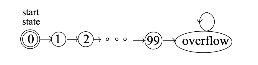
Figure 5.7 State transitions for the 99-bounded counter.

From the course notes Mathematics for Computer Science.

State machines that have at most one transition out of each state is called deterministic. One example is the one above that counts from 1 to 99, and overflows after that. The only transition is from $n$ to $n + 1$.

Note: The general model of a state machine is also about responding to the inputs given, but we are not looking at this for simplicity's sake.

When we used induction the last time, we were showing that a property holds in every step of the process.
A property that is preserved through the whole process is called the preserved invariant.

The invariant principle says that:

If a preserved invariant of a state machine is true for the start state, then it is true for all reachable states.

A reachable state is a state that appears in some execution.
And, what is execution?
It's a sequence of states with the property that:
a) it begins with the start state
b) if $q$ and $r$ are consecutive states, then $q \longrightarrow r$

Realize that the invariant principle is just induction, applied to state machines.

There is a technique called fast exponentiation. Take a look at this code:

base = int(input('Enter base: '))
exp = int(input('Enter exponent: '))

def fast_exp(x, y, z):
    if z < 0: return 'Nonnegative integers only!'
    if z == 0: return y
    if z % 2 == 0:
        return fast_exp(x ** 2, y, z // 2)
    if z % 2 == 1: 
        return fast_exp(x ** 2, x * y, z // 2)

print(fast_exp(base, 1, exp))

Notice that we assume z (the exponent) to be an integer as we use integer division (z // 2) like so.

Here, our start state is (base, 1, exp).

Transitions will be according to this rule:

And, our preserved invariant is that $z$ is a nonnegative integer, and $yx^z = \text{base}^{\text{exp}}$.

One way to verify $yx^z = \text{base}^{\text{exp}}$ is to see if the transitioned state is what we think it is.

Since we're only looking at the case when $z$ is odd, we can use $(z - 1) / 2$ to do the "integer division," and steer clear of a remainder.

In this transition, $y$ becomes $xy$, $x$ becomes $x^2$, and $z$ becomes $(z - 1) / 2$.

In order to write $yx^z$, we have to write $(xy)(x^2)^{(z - 1) / 2}$.

Doing a little simplifying, we get $(xy)x^{z - 1}$, and further simplifying we get $yx^z$ which is indeed what we assumed to be $\text{base}^{\text{exp}}$!
So, the new values of $x$, $y$, and $z$ satisfy the invariant.

To verify a program, there are two properties to look at: partial correctness and termination.

In the fast exponential example, we've proved the correctness, so let's see if we can figure out if it terminates.

One thing to notice is that at each transition, $z$ becomes $\text{quotient}(z, \ 2)$, so it gets smaller. Since it is a nonnegative integer, there is a point where it can't get any smaller, in fact, it can't get smaller more than $log_2(\text{exp})$ times, by then it'd already hit $0$. So, it indeed terminates.

A derived variable is a function assigning a "value" to each state.

So, take a derived variable $v$:

If the values are natural numbers, it can be said that "$v$ is $\mathbb{N}$ valued".

• previous
• next