Conditional Probability

What is the probability that you own a cat, given that you have just bought a cat food?

That's conditional probability, the probability that some event occurs given certain information about it.

Let's suppose that a friend rolls a fair die, and we want to know the probability of rolling 1. The answer is obvious, we have 6 possibilities, and the probability of rolling 1 is $\frac{1}{6}$.

But, now let's say that our friend says that she has rolled an odd number. Now, what's the possibility of rolling 1?
Now that we have our number of possibilities down to three (it can only be 1, 3, or 5), we know that the probability of rolling 1 is $\frac{1}{3}$.

What it shows is that "knowledge" changes probabilities.

If you remember the tree model example in the previous section, it might be recognizable that what we were doing at the last step is using the product rule:

The $\text{Pr}[A]$ is the first branch, and the probability of $B$ given $A$ ($\text{Pr}[B \ | \ A]$) is the second branch. We multiply them to find their intersection.

So, $\text{Pr}[B \ | \ A]$ is the probability of event $B$, given that event $A$ has occurred:

Since we can't divide by $0$, it means that probability of $A$ can't be $0$.

Conditioning on $A$ defines a new probability function $\text{Pr}_A$ where $\text{Pr}_A[\omega] = 0 \ \ \text{if } \omega \notin A$ (probability of an outcome is 0 if that outcome is not in $A$). And, if $\omega \in A$, $\frac{\text{Pr}[\omega]}{\text{Pr}[A]}$.

Let's take a look at what is called the law of total probability.
It is a law for reasoning about probability by cases. If you remember from the (Two) Proof Methods, one of them was Proof by Cases. Breaking up a complicated problem into cases is indeed useful, now let's see how it can be helpful when it comes to probability.

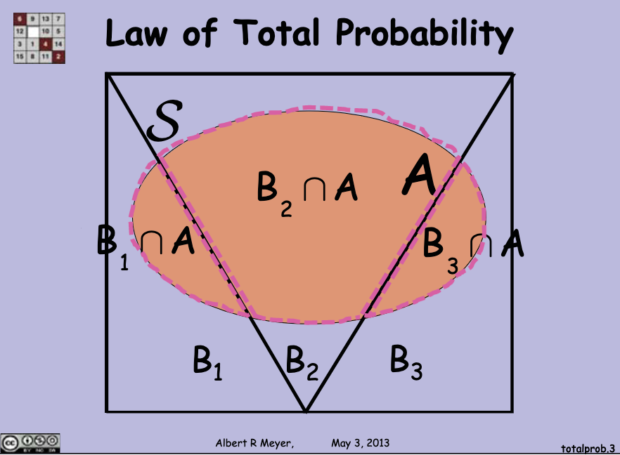
So, let's say that in a sample space $S$, we have a set $A$ which is actually an event. Let's say that we have three more sets $B_1$, $B_2$, and $B_3$ partitioning the sample space, and none of them intersects with each other. Each of these sets has to intersect with $A$, though, so it looks like this:

Since $B_1$, $B_2$, and $B_3$ constitute everything, the union of each of their intersection with $A$ is $A$:

We can add probabilities of those intersections to find the probability of $A$:

Remember the product rule defines an intersection, so we can do a little substitution:

Okay, now it's time to define it better:

If $S$ is a disjoint union of $B_0, \ B_1, \ ...$, then:

$$\text{Pr}[A] = \displaystyle\sum_i \text{Pr}[A \cap B_i]$$

$$= \displaystyle\sum_i \text{Pr}[A \ | \ B_i] \cdot \text{Pr}[B_i]$$

Now, let's look at the famous Bayes' Law.

For example, let's say that two friends are at a café. There are only two options: either coffee or tea (that's a lousy café), and one of them is drinking coffee. What's the probability that both are drinking coffee?

Before using the Bayes' theorem, let's first enumerate all the possibilities.
There are three possibilities, given that one of them is drinking coffee: CC (both are drinking coffee), CT (the first one is drinking coffee and the other is drinking tea), TC (the first one is drinking tea and the other is drinking coffee).

It's obvious that the probability of both of them drinking coffee is $\frac{1}{3}$. We're done.

But, let's now use Bayes' rule.

Let's say that $B$ denotes that both of them are drinking coffee, and $A$ defines that one of them is drinking coffee.
We want $\text{Pr}[B \ | \ A]$, probability of both drinking coffee, given that one of them does.

The formula is $\text{Pr}[B \ | \ A] = \frac{\text{Pr}[A \ | \ B] \cdot \text{Pr}[B]}{\text{Pr}[A]}$.

$\text{Pr}[A \ | \ B]$ is $1$ (if both have coffee, then one of them obviously does have coffee).

$\text{Pr}[B]$ is $\frac{1}{2} \cdot \frac{1}{2} = \frac{1}{4}$ (both of them are drinking coffee with $\frac{1}{2}$ chance).

$\text{Pr}[A]$ is $1 - \frac{1}{4}$ which is $\frac{3}{4}$ (The complement of $\text{Pr}[A]$ is $\frac{1}{4}$).*

The only thing left is to apply the formula:

$\text{Pr}[B \ | \ A] = \frac{1 \cdot \frac{1}{4}}{\frac{3}{4}} = \frac{1}{3}$.

So, the probability of both of them drinking coffee given that one of them does is $\frac{1}{3}$, or $0.33$.

*Not one of them drinking coffee is that they are drinking tea with a $\frac{1}{2}$ chance. So, $\frac{1}{2} \cdot \frac{1}{2} = \frac{1}{4}$.

One thing to note is that the Bayes' theorem allows us to calculate the probability of a prior event given the result of a later event.

Now, let's look at another example from the practice questions of the lecture:

Let $A$ be the event that Albert is giving the lecture.
Let $L$ be the event that Louis goes to the lecture.

$\text{Pr}[A] = 0.8$ and $\text{Pr}[L] = 0.4$.

The probability that Louis goes to lecture given that Albert is giving the lecture ($\text{Pr}[L \ | \ A]$) is $0.3$.

We want to know the probability of Albert giving the lecture given that Louis goes to lecture, that is, $\text{Pr}[A \ | \ L]$.

We have all that we need, so let's plug them into the formula:

$\text{Pr}[A \ | \ L] = \frac{0.3 \ \cdot \ 0.8}{0.4}$

What we have as a result is $0.6$.

One more entertaining example from the practice questions.

This weekend it will rain with probability $\frac{1}{4}$, be sunny with probability $\frac{1}{4}$, and hail baseballs otherwise. If it rains, then there is a 50% chance that I will see a crocodile. If it is sunny, then crocodiles will hide themselves from me with probability $\frac{3}{8}$. If it hails, then I will see a crocodile with complete certainty.

What is the probability I see a crocodile this weekend?

Now, let's look at all the probabilities of seeing a crocodile first.
We have one given that it rains, one given that it is sunny, and one given that it hails.

If it rains (which has a $\frac{1}{4}$ chance), we'll see crocodiles with $\frac{1}{2}$ chance, so multiplying those together we get $\frac{1}{8}$.

If it is sunny (which has a $\frac{1}{4}$ chance), we'll see crocodiles with $\frac{5}{8}$ chance ($1 - \frac{3}{8} = \frac{5}{8}$), so multiplying those together we get $\frac{5}{32}$.

If it hails (which has a $\frac{1}{2}$ chance), we'll see crocodiles with complete certainty, which is $1$.

All we have to do is to add them up together: $\frac{1}{8} + \frac{5}{32} + 1$.

We have the result $\frac{25}{32}$, so we have $0.78125$ chance of seeing crocodiles this weekend.

• previous
• next