Expectation

The expected value of a random variable $R$ is the average value of $R$ where the values are weighted against their probabilities.

So, the expectation of $R$ is the sum of all possible values $v$ times the probability of $R = v$:

It sounds a bit complicated, but let's look at an example that's given in the lecture.

Let's say that we pick a number beforehand, and we roll a dice three times. If we don't get the number we choose, we lose 1 dollar. If the number we choose comes up only once, we win 1 dollar. If it comes up twice, we win 2 dollars, and if all three rolls ends up with our number, we win 3 dollars.

Looking at the probability of each of these three cases, the probability of not getting the number we choose is $\Big(\frac{5}{6}\Big)^3$, which is $\frac{125}{216}$.

The probability of getting our number once is $\binom{3}{1} \big(\frac{5}{6}\big)^2 \big(\frac{1}{6}\big)$.
(Note that the order doesn't matter, we're looking at all possible sequences, that's why it is 3 choose 1 with possibility of one of them being our number and the rest different).

The probability of getting our number twice is similar: $\binom{3}{2} \big(\frac{5}{6}\big) \big(\frac{1}{6}\big)^2$.

Finally, the probability of getting our number all three times is: $\big(\frac{1}{6}\big)^3$.

Let's see what we have for now:

So, if we play 216 games, we expect to never get our number 125 times. We expect to get our number once 75 times, get it twice 15 times, and get it three times only once.

So, on average, what we gain is:

$\frac{125(-1) + 75(1) + 15(2) + 1(3)}{216} = - \frac{17}{216} \approx -8$ cents

That's a negative! Which means that this is not a fair game, we're losing 8 cents on average.
Which means, we expect to lose 8 cents each time we play.

Expectations can be defined alternatively:

So, it is the sum over all the possible outcomes in the sample space of the value of the random variable at that outcome times the probability of that outcome.

In the example, all the possible outcomes in our sample space are the dollar values: -1, 1, 2, or 3. For each of them, we already calculated the probabilities, so the only thing is to multiply each and add them together. Which we did, and find that it was $- \frac{17}{216}$.

This expected value (which was $-8$ in our example) can also be called the mean value, or just mean, or expectation.

Let's look at another example from the practice exercises.

We have a dice that lands on an even number with probability $\frac{1}{4}$. It lands on the values with equal probability. Let's find the expectation of it.

We have 3 even numbers (2, 4, 6), and 3 odd numbers (1, 3, 5) it can land on.

The probability that we get an even number is $\frac{1}{4} \cdot \frac{1}{3} = \frac{1}{12}$.
The probability of we get an odd number is $\frac{3}{4} \cdot \frac{1}{3} = \frac{3}{12} = \frac{1}{4}$.

So, what we'll do is to sum up each value with its probability:
$1(\frac{1}{4}) + 2(\frac{1}{12}) + 3(\frac{1}{4}) + 4(\frac{1}{12}) + 5(\frac{1}{4}) + 6(\frac{1}{12})$, which is equal to $\frac{13}{4} = 3.25$.

The expectation of a binomial distribution ($E[B_{(n, \ p)}]$) is $np$.
Let's look at an example.
All of our coins are fair, and we flip 200 of them. (Or, we flip a fair coin 200 times).
We want to know the expected number of heads.
Well, $n$ is 200, and $p$ is $\frac{1}{2}$. Multiplying them, we have 100.
So, the expected number of heads is 100.

Conditional expectation is defined as:

It is the sum over all possible values that $R$ might take of the probability that $R$ takes that value, given $A$.

An example: let's say we roll a dice. Let $A$ be the probability of getting an even number (one of 2, 4, or 6); let $B$ be the probability of getting a prime number (one of 2, 3, or 5).

Expectation of $A$ given $B$ (expectation of getting an even number given that it is a prime number) is $\frac{1}{3}$.

The law of total expectation is similar to the law of total probability in the sense that it is helpful to reason by cases.
It is defined as:

Let's see how we can use it to calculate the expectation of getting heads in $n$ times of flipping a coin.

Let $e(n)$ be the expected number of heads in $n$ flips.
Then, if the first flip is a head, the expected number of heads is now $1 + e(n - 1)$. So, we have $1$ head and the remaining expectations.

On the other hand, if the first flip is a tail, $e(n)$ is going to be $e(n - 1)$. Because it wasn't heads, what we can look for is the remaining expectations.

These are two cases.

Now, let $p$ be the probability of a head, and $q$ be the probability of a tail.

By total expectation:
$e(n) = \Big([1 + e(n - 1)] \cdot p\Big) + \Big(e(n - 1) \cdot q\Big)$

$q$ is $1 - p$, so replacing it, we get
$e(n) = \Big([1 + e(n - 1)] \cdot p\Big) + \Big(e(n - 1) \cdot (1 - p)\Big)$

Simplifying it further:

$e(n) = p + (p \cdot e(n - 1)) + e(n - 1) - (p \cdot e(n - 1))$

It all simplifies to $e(n) = e(n - 1) + p$.

Look what a beautiful thing we have: $e(n)$ is defined by itself, it is a recursive formula!

So, we need to subtract $1$ from $n$, and add a $p$ (rather, $np$).

Going further, $e(n - 1) = e(n - 2) + 2p$, $...$
So, $e(1) = e(0) + np = np$.
Therefore, the expectation of the number of heads in 1 flip, is just $np$, which is just the probability of getting a head in a flip, which is $\frac{1}{2}$.

The expected time to failure is just the answering how long we have to wait for something.

Let's say we want to get a tail this time, so head will be indicating failure.
Then, the expected time to failure in this case is how long until a head comes up.

Let $p$ be the probability of getting a head ($\text{Pr}[\text{head}]$), let $q$ be the probability of getting a tail, and $F$ be the number of flips until we get the first head.

The probability of getting a head on the first flip ($\text{Pr}[F = 1]$) is just $p$.

The probability of getting a head on the second flip ($\text{Pr}[F = 2]$) is going to be $q \cdot p$ because it means that our first flip resulted in tails.

Note: $PDF_F(n) = q^{n - 1} \cdot p$.

The expected number of flips before we get a head is $\frac{1}{p}$:
$E[F] = \frac{1}{p}$

Why?

Let's look at this tree that we're going to call $B$ that helps us see it:

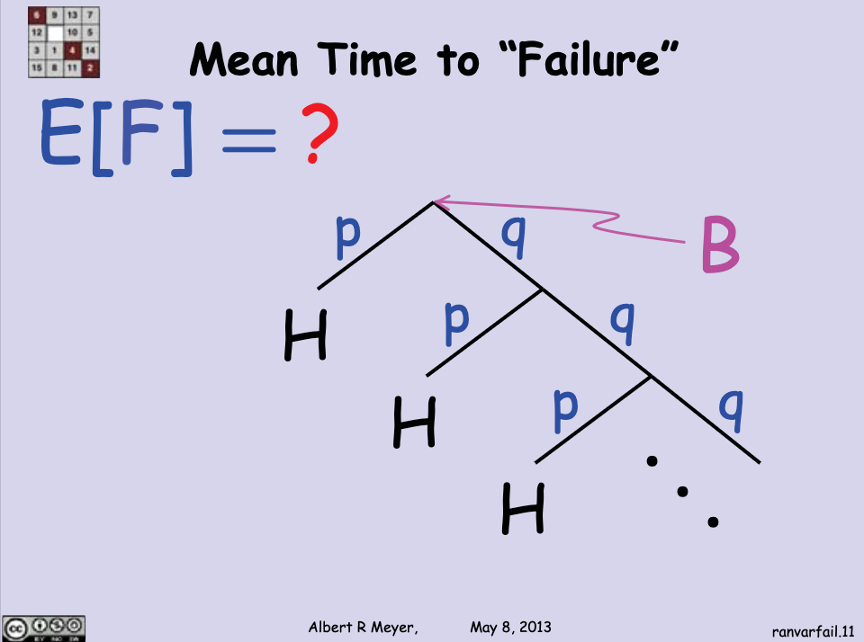
Branches correspond to the act of flipping the coin, so the number of times until we get a head as a result can be counted by following the branches.

This tree is recursive, which means that we can replace a part of it by itself:

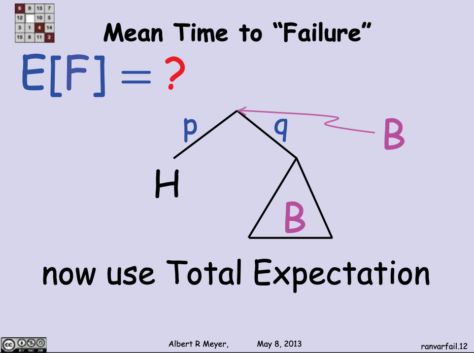
As the slide says, we can use Total Expectation to find $E[F]$, which is just the expected number of branches we have to follow until we reach an $H$.
It will be (the expectation of $F$ given that the first one is a head) times (the probability of getting a head) plus (the expectation of $F$ given that the first one is a tail) times (the probability of getting a tail).

English can be confusing sometimes, so:
$E[F] = E[F \ | \ \text{first = H}] \cdot p + E[F \ | \ \text{first = T}] \cdot q$

Well, the first part (the expected number of flips before getting a head on the first time) is just 1:
$E[F] = 1 \cdot p + E[F \ | \ \text{first = T}] \cdot q$
$E[F] = p + E[F \ | \ \text{first = T}] \cdot q$

The expected number of flips until we get a head given that the first flip resulted in a tail is $1 + E[F]$. Realize that after we get a tail, following the branch going through $q$, we still have the tree $B$ itself. So, we already passed one branch (that's for $1$), and we're still expecting to get a head (that's for $E[F]$), therefore $1 + E[F]$.

Putting it all together, we have $E[F] = p + (1 + E[F]) \cdot q$.

Simplifying it:
$E[F] = p + q + q(E[F])$
$E[F] - q(E[F]) = p + q$

Factoring out $E[F]$:
$E[F](1 - q) = p + q$

Then:
$E[F] = \frac{p + q}{1 - q}$

$q$ can be written as $1 - p$:
$E[F] = \frac{p + (1 - p)}{1 - (1 - p)}$
$E[F] = \frac{1}{p}$

So, the expected number of flips before we get a head is indeed $\frac{1}{p}$.

Two things to note:

• previous
• next