Bite-Sized Mathematics for Computer Science

Notes on MIT's 6.042J

Eda Eren
Table of Contents

Introduction

Prerequisites & Resources

Unit 1: Proofs

00. Introduction to Proofs

01. (Two) Proof Methods

02. The Well Ordering Principle

03. Logic & Propositions

04. Quantifiers and Predicate Logic

05. Sets

06. Binary Relations

07. Induction

08. State Machines — Invariants

09. Recursive Definitions

10. Infinite Sets

Unit 2: Structures

11. GCDs

12. Congruences

13. Euler's Theorem

14. RSA Encryption

15. Digraphs: Walks and Paths

16. Directed Acyclic Graphs

17. Partial Orders and Equivalence

18. Degrees & Isomorphism

19. Coloring & Connectivity

20. Trees

21. Stable Matching

Unit 3: Counting

22. Sums & Products

23. Asymptotics

24. Counting with Bijections

25. Repetitions & Binomial Theorem

26. Pigeonhole Principle, Inclusion-Exclusion

Unit 4: Probability

28. Conditional Probability

29. Independence & Causality

30. Random Variables, Density Functions

31. Expectation

32. Deviation: Markov & Chebyshev Bounds

33. Sampling & Confidence

34. Random Walks & PageRank

Intro to Discrete Probability

It doesn't matter how your relationship with probability theory was in the past, let's look at it with a fresh pair of eyes this time.

What we have in the first place is a set of random outcomes. Some portion of those outcomes (a subset) is an event. What we'll be looking for is the probability of an event:

Probability(event)=number of outcomes in the eventnumber of total outcomes\text{Probability(event)} = \frac{\text{number of outcomes in the event}}{\text{number of total outcomes}}

Before looking at an example, we can keep in mind what is called a 4-part method:

  1. Identify the outcomes
  2. Identify the event
  3. Assign outcome probabilities
  4. Compute event probabilities

Now, let's look at an example from a practice exercise of the course.

Parker has two pairs of black shoes and three pairs of brown shoes. He also has three pairs of red socks, four pairs of brown socks and six pairs of black socks.
Now let's say that Parker chooses a pair of shoes at random and a pair of socks at random. We would like to know the probability of him choosing shoes and socks of the same color.

Let's construct a table to see what we have better:

shoes socks
black 22 66
red 00 33
brown 33 44
TOTAL 55 1313

The first thing we need to do is to identify the outcomes.
In this case, an outcome is a pair of colors.

The second thing to do is to identify the event of interest, to find number of outcomes in the eventnumber of total outcomes\frac{\text{number of outcomes in the event}}{\text{number of total outcomes}}.

The number of total outcomes is 66 (we have two possible colors for shoes—black and brown—, and three possible colors for socks: 23=62 \cdot 3 = 6).

The number of outcomes in the event is 22 because we can only have 2 colors that are in both shoes and socks: black and brown.

Now, the third step is to assign outcome probabilities. We have to do it for everything: So,

Probability of choosing a pair of...
...black shoes:
25\frac{2}{5}
...brown shoes:
35\frac{3}{5}
...black socks:
613\frac{6}{13}
...red socks:
313\frac{3}{13}
...brown socks:
413\frac{4}{13}

The final step is to compute the event probabilities to find the probability that he chooses shoes and socks of the same color.
In order to do that, let's look at the probability tree that is constructed:
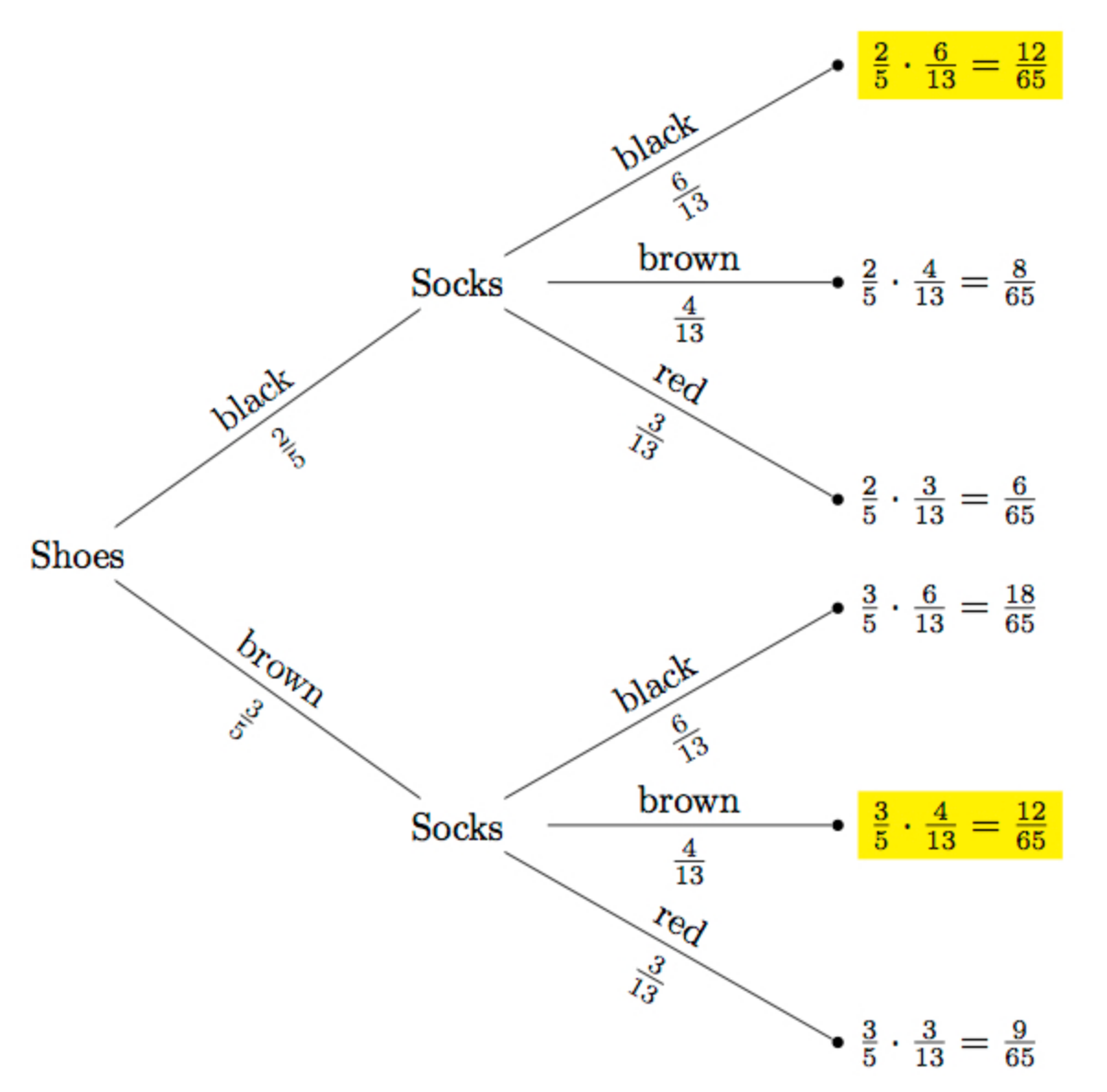
Probability tree

From Q4 Explanation.

Now that we see the probability of choosing black shoes and black socks is 1265\frac{12}{65} and the probability of choosing brown shoes and brown socks is 1265\frac{12}{65}, we can sum the outcomes to find what we're looking for: 1265+1265=2465\frac{12}{65} + \frac{12}{65} = \frac{24}{65}.
So, the probability of choosing the same color of shoes and socks is 2465=0.3692\frac{24}{65} = 0.3692.


Let's look at something called probability spaces.
A probability space consists of two things: a sample space and a probability function.

A sample space is a countable set SS whose elements are called outcomes.

A probability function is a function that assigns probabilities (ranging from 00 to 11 inclusive) to outcomes.
The sum of the probabilities of all the outcomes should add up to 11.
Let SS be the sample space, and ω\omega be an outcome in SS.
So, we should have a probability function Pr:S[0, 1]Pr: S \rightarrow [0, \ 1] such that ωSPr[ω]=1\displaystyle\sum_{\omega \in S} \text{Pr}[\omega] = 1.

The reason of constructing the tree model was to find a probability space.
So, the leaves of the tree correspond to outcomes; and we calculate the outcome probabilities from branch probabilities.

An event is a subset of the sample space, some set of outcomes.
The probability of an event is the sum of the probabilities of all the outcomes in the event:

Pr[E]=ωEPr[ω]\text{Pr}[E] = \displaystyle\sum_{\omega \in E}\text{Pr}[\omega]

From that, we get what is called the sum rule: if we have pairwise disjoint events A0, A1, ...A_0, \ A_1, \ ... (meaning that there are no outcomes in common), the probability of one or more of these events occurring (their union) is the sum of each probability:

Pr[A0A1A2 ...]=Pr[A0]+Pr[A0]+Pr[A1]+Pr[A2]+ ...\text{Pr}[A_0 \cup A_1 \cup A_2 \cup \ ...] = \text{Pr}[A_0] + \text{Pr}[A_0] + \text{Pr}[A_1] + \text{Pr}[A_2] + \ ...

Defined precisely:

Pr[iNAi]=iNPr[Ai]\text{Pr}\Bigg[\bigcup_{i \in \mathbb{N}} A_i\Bigg] = \displaystyle\sum_{i \in \mathbb{N}}\text{Pr}[A_i]

For example, if we have three pairwise disjoint events E0E_0, E1E_1, and E2E_2, each one with the probability of occurring 14\frac{1}{4}.
Then, the probability of any one of them occurring is 0.750.75, because 14+14+14=34=0.75\frac{1}{4} + \frac{1}{4} + \frac{1}{4} = \frac{3}{4} = 0.75.


Now let's define some rules:

The difference rule:
Pr[AB]=Pr[A]Pr[AB]\text{Pr}[A - B] = \text{Pr}[A] - \text{Pr}[A \cap B]
By the sum rule: Pr[A]=Pr[AB]+Pr[AB]\text{Pr}[A] = \text{Pr}[A \cap B] + \text{Pr}[A - B]. Substituting it, we are left with Pr[AB]=Pr[AB]\text{Pr}[A - B] = \text{Pr}[A - B].
The inclusion-Exclusion:
Pr[AB]=Pr[A]+Pr[B]Pr[AB]\text{Pr}[A \cup B] = \text{Pr}[A] + \text{Pr}[B] - \text{Pr}[A \cap B]
This is similar to what we have seen in this section.
The union bound:
Pr[AB]Pr[A]+Pr[B]\text{Pr}[A \cup B] \leq \text{Pr}[A] + \text{Pr}[B]
This can be understood from the inclusion-exclusion of two sets, clearly it is defined as the sum of the probabilities of two sets minus the probability of their intersection. So, it has to be less than the sum of their probabilities.
The monotonicity:
Pr[A]Pr[AB]\text{Pr}[A] \leq \text{Pr}[A \cup B]